Week 4, Day 2 (Temporal-Difference Methods)
Welcome to second day (Week 4) of the McE-51069 course.
Lecture Notebook
You can download the notebook for today lecture from this link.
Temporal-Difference Learning
In this notebook, we will learn Temporal-Difference (TD) Methods using CliffWalking environment from OpenAI Gym. You can find more about this environment here.
CliffWalking Env
Lets explore gym CliffWalking environment. We begin by importing the necessary modules and packages.
import sys
import gym
import numpy as np
from collections import defaultdict, deque
import seaborn as sns
import matplotlib.pyplot as plt
%matplotlib inline
We can create an instance of the CliffWalking env by calling gym.make('CliffWalking-v0').
env = gym.make('CliffWalking-v0')
Now, lets find the details information of observation and action spaces.
env.observation_space
env.action_space
CliffWalking environment is adapted from example (6.6) of Sutton and Barto text book.
Observation space (State) is 4x12 matrix, with (using NumPy matrix indexing):
[[ 0,  1,  2,  3,  4,  5,  6,  7,  8,  9, 10, 11],
 [12, 13, 14, 15, 16, 17, 18, 19, 20, 21, 22, 23],
 [24, 25, 26, 27, 28, 29, 30, 31, 32, 33, 34, 35],
[36, 37, 38, 39, 40, 41, 42, 43, 44, 45, 46, 47]]- [3, 0] as the start at bottom-left (state
36) - [3, 11] as the goal at bottom-right (state
47) - [3, 1..10] as the cliff at bottom-center (states
37 to 46)
Action space consists of four discrete values.
- 0 =
UP - 1 =
RIGHT - 2 =
DOWN - 3 =
LEFT
This CliffWalking environment information is documented in the source code as follows:
Each time step incurs -1 reward, and stepping into the cliff incurs -100 reward and a reset to the start. An episode terminates when the agent reaches the goal.
Optimal policy of the environment is shown below.
[[ 0,  1,  2,  3,  4,  5,  6,  7,  8,  9, 10, 11],
 [12, 13, 14, 15, 16, 17, 18, 19, 20, 21, 22, 23],
 [ >,  >,  >,  >,  >,  >,  >,  >,  >,  >,  >,  >],
 [ S, 37, 38, 39, 40, 41, 42, 43, 44, 45, 46,  G]]
Run the code cell below to know more about the CliffWalking environment.
# initialize the env
state = env.reset()

while True:

    for i in range(2):
        action = env.action_space.sample()
        print(f"Current state {i}: ",state)
        print(f"Current action {i}: ",action)
        state, reward, done, info = env.step(action)
        print(f"Reward {i+1}: ",reward)
        env.render()

    break
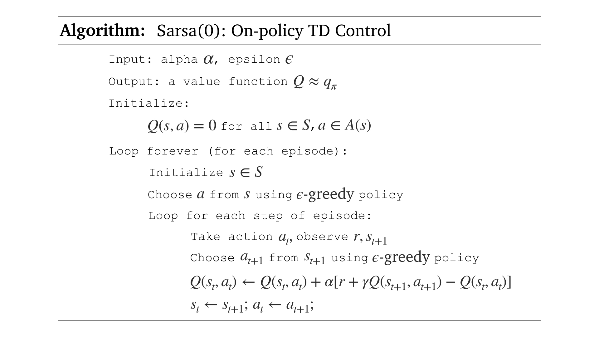
Sarsa: On-policy TD Control
Lets start learning TD methods by implementing Sarsa(0), which is an on-policy TD Control method. The pseudocode below is used to implement the algorithm.
We will call this function sarsa.
The function accepts five input arguments:
-
env: an instance of OpenAI Gym's CliffWalking environment -
num_of_episodes: number of episodes to play -
alpha: step-size parameter in update equation -
plot_every: store average scores over n episodes -
gamma: discount rate (default = 1.0)
The function returns two outputs:
-
Q: Q-Table of state, action pairs $Q(s,a)$ -
avg_scores: average scores for visualizing
def epsilon_greedy_action(epsilon, number_of_actions, Q):

    policy = np.ones(number_of_actions) * epsilon / number_of_actions
    max_action_index = np.argmax(Q)
    policy[max_action_index] = 1 - epsilon + (epsilon / number_of_actions)
    action = np.random.choice(np.arange(number_of_actions), p=policy)

    return action


def sarsa(env, num_of_episodes, alpha, plot_every=100, gamma=1.0):

    # initialize empty dictionary Q
    Q = defaultdict(lambda: np.zeros(env.action_space.n))

    # monitor performance
    tmp_scores = deque(maxlen=plot_every)
    avg_scores = deque(maxlen=num_of_episodes)

    for i in range(1, num_of_episodes+1):

        score = 0

        # initialize the episode
        s = env.reset()

        # calculate epsilon value
        epsilon = 1 / i

        # epsilon-greedy policy action selection
        a = epsilon_greedy_action(epsilon, env.action_space.n, Q[s])

        # run until episode terminates
        while True:

            ##############################
            # take action A, observe R,S'
            ##############################
            next_s, reward, done, info = env.step(a)
            score += reward

            ################################################
            # choose A' from S' using epsilon-greedy policy
            ################################################
            next_a = epsilon_greedy_action(epsilon, env.action_space.n, Q[next_s])

            #######################################################
            # Q(s,a) <- Q(s,a) + alpha*[R+gamma*Q(s',a') - Q(s,a)]
            #######################################################
            td_target = reward + gamma*Q[next_s][next_a]
            Q[s][a] = Q[s][a] + alpha*(td_target - Q[s][a])

            ###################
            # s <- s'; a <- a'
            ###################
            s = next_s
            a = next_a

            if done:
                tmp_scores.append(score)
                break

        if (i % plot_every == 0):
            avg_scores.append(np.mean(tmp_scores))
            if (i % 1000 == 0):
                print(f"Episode {i}/{num_of_episodes}: Average Reward: {np.max(avg_scores)}")

    return Q, avg_scores
Run the code cell below to train the agent. Feel free to tune the hyperparameters to get the optimal action-value function.
env.seed(0)
np.random.seed(0)

# Hyperparameters
num_of_episodes = 5000
alpha = 0.012
plot_every = 100
gamma = 1.0

Q, avg_scores = sarsa(env, num_of_episodes, alpha,
                      plot_every, gamma)

# plot performance
plt.plot(np.linspace(0,num_of_episodes,len(avg_scores),endpoint=False),
         np.asarray(avg_scores), 'r')

plt.xlabel('Episode Number')
plt.ylabel('Average Reward (Over Next %d Episodes)' % plot_every)
plt.grid(True)
plt.show()

We can plot the corressponding action-value function by running code cell below.
# obtain the corresponding state-value function
V = np.array([np.max(Q[key]) if key in Q else -1 for key in np.arange(48)]).reshape(4, 12)

fig = plt.figure(figsize=(12,6))

plt.title('State-Value Function')
sns.heatmap(V, cmap="YlGnBu", cbar=False, annot=True, xticklabels=[], yticklabels=[])
plt.show()

# print the estimated optimal policy
policy = np.array([np.argmax(Q[key]) if key in Q else -1 for key in np.arange(48)]).reshape((4,12))
print("\nEstimated Optimal Policy (UP = 0, RIGHT = 1, DOWN = 2, LEFT = 3, N/A = -1):")
print(policy)
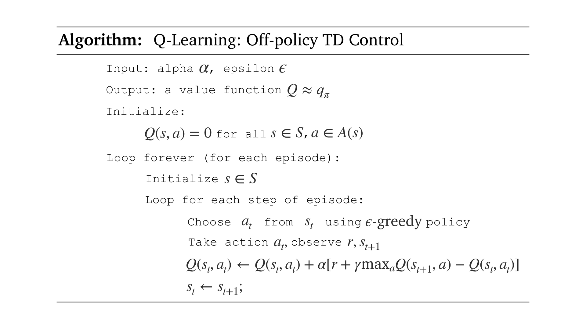
Q-learning: Off-policy TD Control
We will move to the Sarsamax algorithm, also known as Q-Learning, which is an off-policy TD Control algorithm. In this case, the learned action-value function $Q$ directly estimates $q_*$, the optimal action-value function, independent of the policy being followed.
We will use the pseudocode below to implement our Q-Learning algorithm.
We will call this function qlearning.
The function accepts five input arguments:
-
env: an instance of OpenAI Gym's CliffWalking environment -
num_of_episodes: number of episodes to play -
alpha: step-size parameter in update equation -
plot_every: store average scores over n episodes -
gamma: discount rate (default = 1.0)
The function returns two outputs:
-
Q: Q-Table of state, action pairs $Q(s,a)$ -
avg_scores: average scores for visualizing
def qlearning(env, num_of_episodes, alpha, plot_every=100, gamma=1.0):

    # initialize empty dictionary Q
    Q = defaultdict(lambda: np.zeros(env.action_space.n))

    # monitor performance
    tmp_scores = deque(maxlen=plot_every)
    avg_scores = deque(maxlen=num_of_episodes)

    for i in range(1, num_of_episodes+1):

        score = 0

        # initialize the episode
        s = env.reset()

        # calculate epsilon value
        epsilon = 1 / i

        # run until episode terminates
        while True:

            ##############################################
            # choose A from S using epsilon-greedy policy
            ##############################################
            a = epsilon_greedy_action(epsilon, env.action_space.n, Q[s])

            ##############################
            # take action A, observe R,S'
            ##############################
            next_s, reward, done, info = env.step(a)
            score += reward

            #######################################################
            # Q(s,a) <- Q(s,a) + alpha*[R+gamma*max_aQ(s',a) - Q(s,a)]
            #######################################################
            td_target = reward + gamma*np.max(Q[next_s])
            Q[s][a] = Q[s][a] + alpha*(td_target - Q[s][a])

            ##########
            # s <- s'
            ##########
            s = next_s

            if done:
                tmp_scores.append(score)
                break

        if (i % plot_every == 0):
            avg_scores.append(np.mean(tmp_scores))
            if (i % 1000 == 0):
                print(f"Episode {i}/{num_of_episodes}: Average Reward: {np.max(avg_scores)}")

    return Q, avg_scores
env.seed(0)
np.random.seed(0)

# Hyperparameters
num_of_episodes = 5000
alpha = 0.012
plot_every = 100
gamma = 1.0

Q, avg_scores = qlearning(env, num_of_episodes, alpha,
                      plot_every, gamma)

# plot performance
plt.plot(np.linspace(0,num_of_episodes,len(avg_scores),endpoint=False),
         np.asarray(avg_scores), 'r')

plt.xlabel('Episode Number')
plt.ylabel('Average Reward (Over Next %d Episodes)' % plot_every)
plt.grid(True)
plt.show()

# obtain the corresponding state-value function
V = np.array([np.max(Q[key]) if key in Q else -1 for key in np.arange(48)]).reshape(4, 12)

fig = plt.figure(figsize=(12,6))

plt.title('State-Value Function')
sns.heatmap(V, cmap="YlGnBu", cbar=False, annot=True, xticklabels=[], yticklabels=[])
plt.show()

# print the estimated optimal policy
policy = np.array([np.argmax(Q[key]) if key in Q else -1 for key in np.arange(48)]).reshape((4,12))
print("\nEstimated Optimal Policy (UP = 0, RIGHT = 1, DOWN = 2, LEFT = 3, N/A = -1):")
print(policy)