Week 4, Day 1 (Introduction to Reinforcement Learning Framework)
Welcome to first day (Week 4) of the McE-51069 course.
Lecture Notebook
You can download the notebooks file for today lecture here.

Introduction to OpenAI Gym
Gym is a toolkit for developing and comparing reinforcement learning algorithms. It supports teaching agents everything from walking to playing games like Pong or Pinball. It makes no assumptions about the structure of your agent, and is compatible with any numerical computation library, such as TensorFlow or Theano.
!pip install gym
Gym Environments
The OpenAI Gym involves a diverse suite of physical simulation environments ranging from easy to challenging tasks that we can play with and test our reinforcement learning algorithms with it. These include Classic control games, Atari, MuJoCo, Robotics and much more. You can find more about gym environments here.
In this course, we will focus on Toy text, Classic control and Atari environments.
Classic control and Toy text
These environments include small-scale tasks, mostly from the RL literature.


Creating your first environment
We can simply call gym.make("env_name") to create an environment object. Here "env_name" denotes the name of the environment we are calling. All the available names of the environments can be found here.
# importing openai gym library
import gym
import numpy as np

# create classic cart-pole env
env = gym.make('MountainCar-v0')

# reset/initialize the env
env.reset()

for _ in range(200):
    env.step(env.action_space.sample()) # take a random action
    env.render() # render the environment

# close the rendering
env.close()
We can interact with the environment by two main methods:
env.reset()-
env.step(action)obs = env.reset()method initialize and returns an initial observation (or state) of the environment. We will learn more about gym observations later.
obs_next, reward, done, info = env.step(action)method interacts with the environment by taking an action as an input and returns four values:obs_next(env.observation_space), reward(float), done(bool) and info(dict).
Spaces
Every gym environment comes with an action_space and an observation_space. The formats of action and observation of an environment are defined by env.action_space and env.observation_space respectively, which are of type Space.
Types of gym spaces:
-
gym.spaces.Discrete(n): fixed range of non-negative discrete numbers from 0 to n-1. -
gym.spaces.Box: represents an n-dimensional box, where the upper and lower bounds of each dimension are defined byBox.lowandBox.high.
Lets explore these two spaces.
# import spaces module from gym
from gym import spaces

space = spaces.Discrete(8) # Set with 8 elements {0, 1, 2, ..., 7}

space
space.sample()
import warnings

low_value = np.array([0,0,-1])
high_value = np.array([1,1,1])

box = spaces.Box(low_value, high_value)

box
box.low
box.high
We can now check what are the spaces of previous cart-pole example used. You can find more about the spaces of cart-pole environment here.
env = gym.make('CartPole-v0')

print(env.action_space)

print(env.observation_space)
env.observation_space.low
env.observation_space.high

Monte Carlo Methods
In this notebook, we will learn Monte Carlo Methods using Blackjack environment from OpenAI Gym. You can find more about this environment here.
import gym
import numpy as np
from collections import defaultdict
import seaborn as sns
import matplotlib.pyplot as plt
from matplotlib.colors import LinearSegmentedColormap
from utilities import plot_v, plot_policy
We can create an instance of the blackjack env by calling gym.make('Blackjack-v0').
env = gym.make('Blackjack-v0')
Now, lets find the details information of observation and action spaces.
env.observation_space
env.action_space
Observation space (State) is a tuple of three discrete spaces. You can find the details information of the observation space of blackjack env here.
- the players current sum $\in \{0, 1, \ldots, 31\}$
- the dealer's one showing card $\in \{1, 2, \ldots, 10\}$
- the player holds a usable ace or not (0 =
falseor 1 =true)
Action space consists of two discrete values. You can find the details information of the action space of blackjack env here.
- 0 =
STICK - 1 =
HIT
Before training our agent with Monte Carlo Methods, lets play blackjack with a random policy.
# number of episodes to play
num_of_games = 2

for episode in range(num_of_games):

    # initialize the env
    state = env.reset()
    while True:

        # print current observation state
        print(state)

        # select action (hit or stick) randomly
        action = env.action_space.sample()

        # interacts with the env
        state, reward, done, info = env.step(action)

        # break loop if wins or lose
        if done:
            print('End game! Reward: ', reward)
            print('You won :)\n') if reward > 0 else print('You lost :(\n')
            break
We will closely follow the example (5.1) of Sutton and Barto text book.
We begin by considering a policy that
sticksif the player's sum is 20 or 21, and otherwisehits.
The following function implements this policy. The function accepts an instance of OpenAI Gym's Blackjack environment as an input and returns an episode as an output which is a list of (state, actions and rewards) tuples.
def play_single_episode(env):

    episode = []
    state = env.reset()

    while True:
        # custom policy
        action = 0 if state[0] >= 20 else 1

        next_state, reward, done, info = env.step(action)
        episode.append((state, action, reward)) # (S0, A0, R1), (S1, A1, R2), ...
        state = next_state

        if done:
            break
    return episode
Lets play Blackjack with the implemented policy.
env = gym.make('Blackjack-v0')

num_of_games = 3
for i in range(num_of_games):
    print(play_single_episode(env))
Now, we are ready to implement our MC Prediction algorithm. We will start with Every-Visit MC Prediction, which is easier to understand and implement. The pseudocode below is used to implement our algorithm.
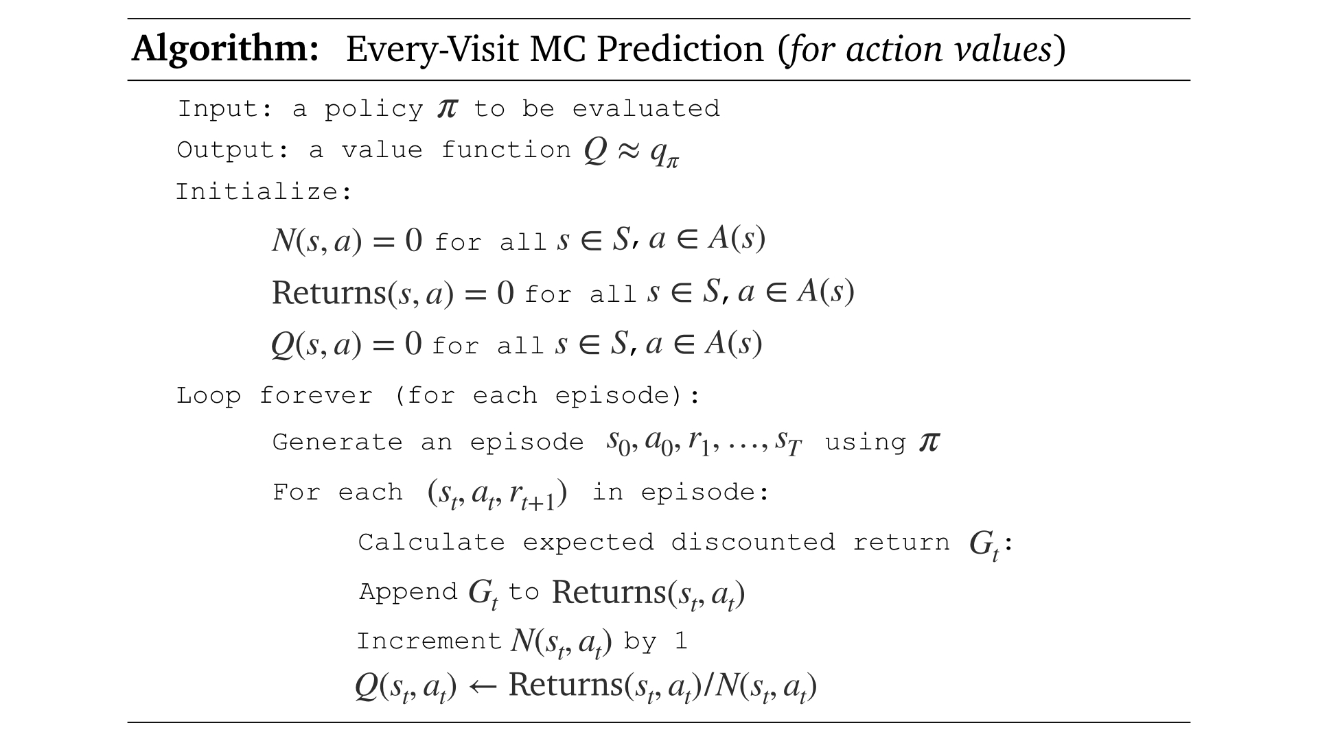
We will call this function every_visit_mc_prediction.
The function accepts four input arguments:
-
env: an instance of OpenAI Gym's Blackjack environment -
num_of_episodes: number of episodes to play -
episode_generator: generate an episode of $(S_{i-1}, A_{i-1} , R_i)$ tuples using custom policy -
gamma: discount rate (default = 1.0)
The function returns an action-value:
-
Q: Q-Table of state, action pairs $Q(s,a)$
def every_visit_mc_prediction(env, num_of_episodes, episode_generator, gamma=1.0):

    # initialize empty dictionaries of arrays
    N = defaultdict(lambda: np.zeros(env.action_space.n))
    Q = defaultdict(lambda: np.zeros(env.action_space.n))
    Returns = defaultdict(lambda: np.zeros(env.action_space.n))

    for i in range(1, num_of_episodes+1):
        # generate a single episode (S0, A0, R1,..., ST, AT, RT)
        episode = episode_generator(env)

        # for each tuple in episode
        for i, (s, a, r) in enumerate(episode):

            # calculate expected discounted return G
            # from current state onwards
            G = sum([x[2]*(gamma**i) for i,x in enumerate(episode[i:])])

            Returns[s][a] += G
            N[s][a] += 1.0
            Q[s][a] = Returns[s][a] / N[s][a]

    return Q
Lets run our Every-Visit MC Prediction algorithm. Set the desired number of episodes.
env.seed(0)
num_of_episodes = 10000

# run every-visit mc prediction algorithm for n episodes
Q = every_visit_mc_prediction(env, num_of_episodes, play_single_episode)
Now, lets plot our predicted state-value function using our test policy.
# obtain the corresponding state-value function for our test policy
V = dict((k, (k[0]>=20)*v[0] + (k[0]<20)*v[1]) for k, v in Q.items())

# plot the state-value function heatmap
plot_v(V)

We can also test the First-Visit MC Prediction algorithm by using the pseudocode provided below.
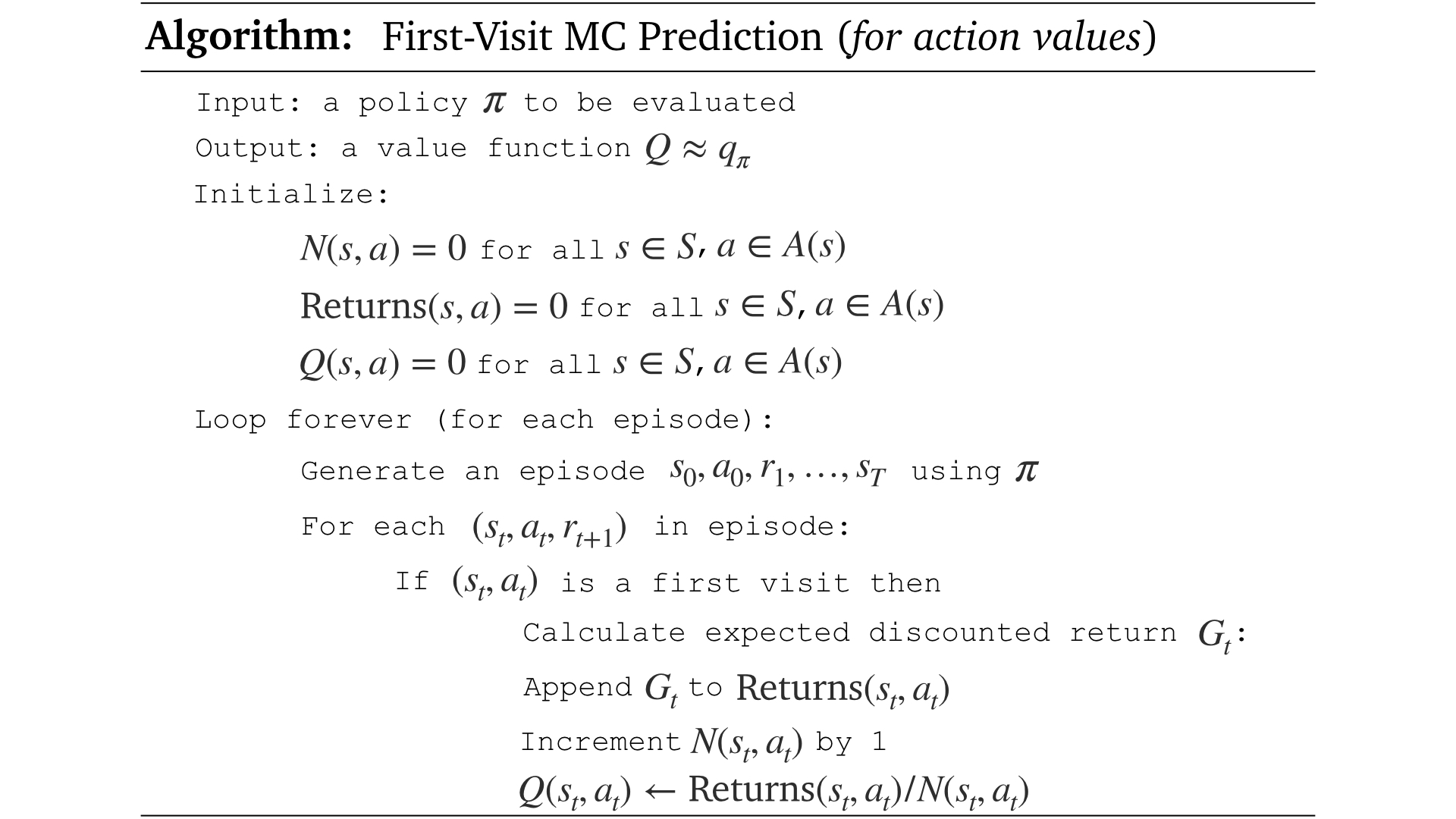
We will call this function first_visit_mc_prediction.
def first_visit_mc_prediction(env, num_of_episodes, episode_generator, gamma=1.0):

    # initialize empty dictionaries of arrays
    N = defaultdict(lambda: np.zeros(env.action_space.n))
    Q = defaultdict(lambda: np.zeros(env.action_space.n))
    Returns = defaultdict(lambda: np.zeros(env.action_space.n))

    for i in range(1, num_of_episodes+1):
        # generate a single episode (S0, A0, R1,..., ST, AT, RT)
        episode = episode_generator(env)

        # create first-visit-check set
        first_visit_check = set()

        # for each tuple in episode
        for i, (s, a, r) in enumerate(episode):

            # if s is already in visit-check set
            if s in first_visit_check:
                # skip this state
                continue

            # add state to set
            first_visit_check.add(s)

            # calculate expected discounted return G
            # from current state onwards
            G = sum([x[2]*(gamma**i) for i,x in enumerate(episode[i:])])

            Returns[s][a] += G
            N[s][a] += 1.0
            Q[s][a] = Returns[s][a] / N[s][a]

    return Q

env.seed(0)
num_of_episodes = 10000

# run every-visit mc prediction algorithm for n episodes
Q = first_visit_mc_prediction(env, num_of_episodes, play_single_episode)
# obtain the corresponding state-value function for our test policy
V = dict((k, (k[0]>=20)*v[0] + (k[0]<20)*v[1]) for k, v in Q.items())

# plot the state-value function heatmap
plot_v(V)
Monte Carlo Control
We just finish the first step in Generalized Policy Iteration (GPI), which is a Policy Evaluation step. We do this by implementing two different MC prediction algorithms. Lets move to the next step where we will improve our policy.
In this notebook, we will implement Every-Visit Constant-$\alpha$ MC Control algorithm.
number_of_actions = 4

policy = np.ones(number_of_actions) * 1/number_of_actions

print("Initial Policy: ",policy)
# Choose epsilon value
epsilon = 1

# for all actions
policy = np.ones(number_of_actions) * epsilon / number_of_actions

print(policy)
# only for maximum action
max_action = 3
policy[max_action] = 1 - epsilon + (epsilon / number_of_actions)

print(policy)
np.random.choice(np.arange(number_of_actions), p=policy)
We will call this function epsilon_greedy_action.
The function accepts three input arguments:
-
epsilon(value between 0 and 1) -
number_of_actions(action space size) -
Q(Action-Value function)
The function returns action index, which is chosen using the epsilon-greedy policy.
def epsilon_greedy_action(epsilon, number_of_actions, Q):

    policy = np.ones(number_of_actions) * epsilon / number_of_actions
    max_action_index = np.argmax(Q)
    policy[max_action_index] = 1 - epsilon + (epsilon / number_of_actions)
    action = np.random.choice(np.arange(number_of_actions), p=policy)

    return action
Lets implement similar episode generator function from MC Prediction using our epsilon-greedy policy.
def play_single_episode(env, Q, epsilon):

    episode = []
    state = env.reset()

    while True:
        # epsilon-greedy policy
        action = epsilon_greedy_action(epsilon, env.action_space.n, Q[state])

        next_state, reward, done, info = env.step(action)
        episode.append((state, action, reward)) # (S0, A0, R1), (S1, A1, R2), ...
        state = next_state

        if done:
            break
    return episode
Every-Visit Constant-$\alpha$ MC Control
Now, we are ready to implement the Every-Visit Constant-$\alpha$ MC Control algorithm. The pseudocode below is used to implement our algorithm.
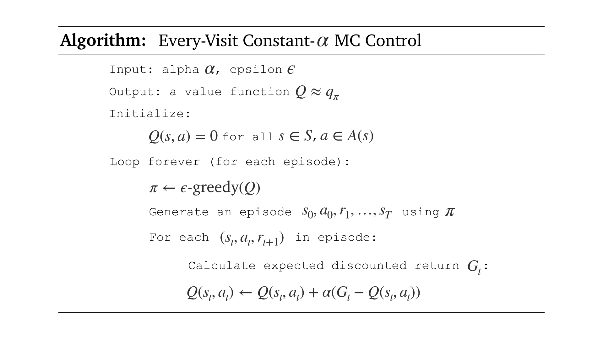
We will call this function every_visit_mc_control.
The function accepts eight input arguments:
-
env: an instance of OpenAI Gym's Blackjack environment -
num_of_episodes: number of episodes to play -
episode_generator: generate an episode of $(S_{i-1}, A_{i-1} , R_i)$ tuples using epsilon-greedy policy -
alpha: step-size parameter in update equation -
gamma: discount rate (default = 1.0) -
epsilon: epsilon value for policy (default = 1.0) -
epsilon_decay: decay rate of the epsilon (default = 0.99999) -
epsilon_min: minimum value of the epsilon (default = 0.05)
The function returns an action-value:
-
Q: Q-Table of state, action pairs $Q(s,a)$
def every_visit_mc_control(env, num_of_episodes, episode_generator, alpha,
                           gamma=1.0, epsilon=1.0,
                           epsilon_decay=0.99999, epsilon_min=0.05):

    # initialize empty dictionary Q
    Q = defaultdict(lambda: np.zeros(env.action_space.n))

    for i in range(1, num_of_episodes+1):

        # calculate epsilon value
        epsilon = max(epsilon*epsilon_decay, epsilon_min)

        # generate a single episode (S0, A0, R1,..., ST, AT, RT)
        # using epsilon-greedy policy
        episode = episode_generator(env, Q, epsilon)

        # for each tuple in episode
        for i, (s, a, r) in enumerate(episode):

            # calculate expected discounted return G
            # from current state onwards
            G = sum([x[2]*(gamma**i) for i,x in enumerate(episode[i:])])

            Q[s][a] = Q[s][a] + alpha*(G - Q[s][a])

    return Q

# Hyperparameters
num_of_episodes = 10000
alpha = 0.01
gamma = 1.0
epsilon = 1.0
epsilon_decay = 0.9999
epsilon_min = 0.09

# run every-visit constant-alpha mc control algorithm
Q = every_visit_mc_control(env, num_of_episodes, play_single_episode, alpha,
                           gamma, epsilon, epsilon_decay, epsilon_min)
# obtain the corresponding state-value function
V = dict((k,np.max(v)) for k, v in Q.items())

# plot the state-value function heatmap
plot_v(V)

# obtain the corresponding best policy
policy = dict((k,np.argmax(v)) for k, v in Q.items())

# plot the state-value function heatmap
plot_policy(policy)

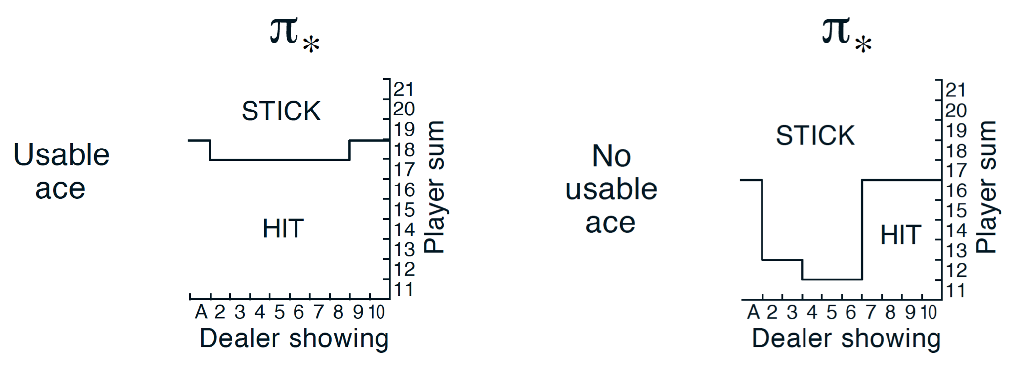
We can refer to Figure 5.2 of the Sutton and Barto text book for true optimal policy which is shown below. Feel free to tweak around the hyperparameters and compare your results with the true optimal policy.