Week 3, Day 1 (Dataset Preparation and Arrangement)
Welcome to first day (Week 3) of the McE-51069 course.
- Datasets
You can download resources for today from this link. We have also posted a guide video on downloading and accessing materials on youtube channel.
Datasets comes in different forms from various sources. So the question here is what exactly is a dataset and how do we handle datasets for machine learning? To experiment the conditions, we must first know how to manipulate a dataset.
Pandas is a python library for data manipulation and analysis. In this section, we will feature a brief introuction to pandas.
import pandas as pd
import numpy as np
import matplotlib.pyplot as plt
import cv2
import math
%matplotlib inline
Pandas stores data in dataframe objects. We can assign columns to each to numpy array (or) list to create a dataframe.
names = ['Jack','Jean','Jennifer','Jimmy']
ages = np.array([23,22,24,21])
# print(type(names))
# print(type(ages))

df = pd.DataFrame({'name': names,
                   'age': ages,
                   'city': ['London', 'Berlin', 'New York', 'Sydney']},index=None)

df.head()
# df.style.hide_index()
Now, let's see some handy dataframe tricks.
df[['name','city']]
df.info()
# print(df.columns)
# print(df.age)
Now that we know how to create a dataframe, we can save the dataframe we created.
df.to_csv('Ages_and_cities.csv',index=False,header=True)
df = pd.read_csv('Ages_and_cities.csv')
df.head()
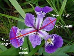
In this section, we used Iris flowers dataset, which contains petal and sepal measurements of three species of Iris flowers.
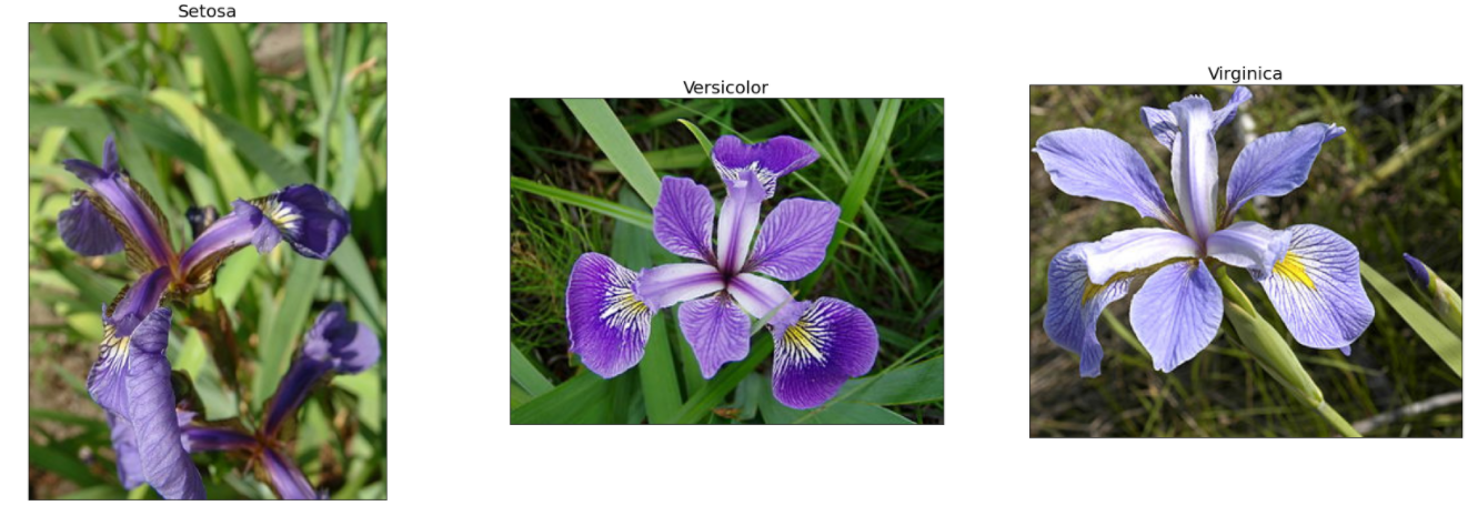
This dataset was introduced by biologist Ronald Fisher in his 1936 paper. The following figure explains the way length and width are mesured or petal and speal of each flower.
When we observe the dataset, we will discover that the dataset has four features and three unique labels for three flowers.
df = pd.read_csv('iris_data.csv')
df.head()
# df.head(3)
df.tail()
Now that we understand our dataset, let's prepare to seperate our data based on labels for unique visualization.
df.loc[80:85,("sepal_length","variety")]
# df.iloc[80:85,2:5]
df.iloc[80:85,[0,4]]
Se= df.loc[df.variety =='Setosa', :]
Vc= df.loc[df.variety =='Versicolor', :]
Vi= df.loc[df.variety =='Virginica', :]
Vi.head()
df = pd.read_csv('iris_data.csv')
# df.dtypes
First, we will visualize each measurement with histograms to observe the output distribution for each class.
plt.figure(figsize=(15,15))

plt.subplot(2, 2, 1)
plt.hist(Se.sepal_length,bins=15,color="steelblue",edgecolor='black',alpha =0.4, label="Setosa")
plt.hist(Vc.sepal_length,bins=15,color='red',edgecolor='black', alpha =0.3, label="Versicolor")
plt.hist(Vi.sepal_length,bins=15,color='blue',edgecolor='black', alpha =0.3, label="Virginica")
plt.title("sepal length distribution"), plt.xlabel('cm')
plt.legend()

plt.subplot(2, 2, 2)
plt.hist(Se.sepal_width,bins=15,color="steelblue",edgecolor='black',alpha =0.4, label="Setosa")
plt.hist(Vc.sepal_width,bins=15,color='red',edgecolor='black', alpha =0.3, label="Versicolor")
plt.hist(Vi.sepal_width,bins=15,color='blue',edgecolor='black', alpha =0.3, label="Virginica")
plt.title("sepal width distribution"), plt.xlabel('cm')
plt.legend()

plt.subplot(2, 2, 3)
plt.hist(Se.petal_length,bins=10,color="steelblue",edgecolor='black',alpha =0.4, label="Setosa")
plt.hist(Vc.petal_length,bins=10,color='red',edgecolor='black', alpha =0.3, label="Versicolor")
plt.hist(Vi.petal_length,bins=10,color='blue',edgecolor='black', alpha =0.3, label="Virginica")
plt.title("petal length distribution"), plt.xlabel('cm')
plt.legend()

plt.subplot(2, 2, 4)
plt.hist(Se.petal_width,bins=10,color="steelblue",edgecolor='black',alpha =0.4, label="Setosa")
plt.hist(Vc.petal_width,bins=10,color='red',edgecolor='black', alpha =0.3, label="Versicolor")
plt.hist(Vi.petal_width,bins=10,color='blue',edgecolor='black', alpha =0.3, label="Virginica")
plt.title("petal width distribution"), plt.xlabel('cm')
plt.legend()

Now, we will visualize multiple features with scatter plots to gain some more insights.
plt.figure(figsize=(15,15))

area = np.pi*20

plt.subplot(2, 2, 1)
plt.scatter(Se.sepal_length,Se.sepal_width, s=area, c="steelblue", alpha=0.6, label="Setosa")
plt.scatter(Vc.sepal_length,Vc.sepal_width, s=area, c="red", alpha=0.6, label="Versicolor")
plt.scatter(Vi.sepal_length,Vi.sepal_width, s=area, c="blue", alpha=0.5, label="Virginica")
plt.title("sepal length Vs sepal width"), plt.xlabel('cm'), plt.ylabel('cm')
plt.legend()

plt.subplot(2, 2, 2)
plt.scatter(Se.petal_length,Se.petal_width, s=area, c="steelblue", alpha=0.6, label="Setosa")
plt.scatter(Vc.petal_length,Vc.petal_width, s=area, c="red", alpha=0.6, label="Versicolor")
plt.scatter(Vi.petal_length,Vi.petal_width, s=area, c="blue", alpha=0.5, label="Virginica")
plt.title("petal length Vs petal width"), plt.xlabel('cm'), plt.ylabel('cm')
plt.legend()

plt.subplot(2, 2, 3)
plt.scatter(Se.sepal_length,Se.petal_length, s=area, c="steelblue", alpha=0.6, label="Setosa")
plt.scatter(Vc.sepal_length,Vc.petal_length, s=area, c="red", alpha=0.6, label="Versicolor")
plt.scatter(Vi.sepal_length,Vi.petal_length, s=area, c="blue", alpha=0.5, label="Virginica")
plt.title("sepal length Vs petal length"), plt.xlabel('cm'), plt.ylabel('cm')
plt.legend()

plt.subplot(2, 2, 4)
plt.scatter(Se.sepal_width,Se.petal_width, s=area, c="steelblue", alpha=0.6, label="Setosa")
plt.scatter(Vc.sepal_width,Vc.petal_width, s=area, c="red", alpha=0.6, label="Versicolor")
plt.scatter(Vi.sepal_width,Vi.petal_width, s=area, c="blue", alpha=0.5, label="Virginica")
plt.title("sepal width Vs petal width"), plt.xlabel('cm'), plt.ylabel('cm')
plt.legend()

We can definitely see some blobs forming from these visualizations. "Setosa" class unsally stands out from the other two classes but the sepal width vs sepal length plot shows "versicolor" and "virginica" classes will more challenging to classify compared to "setosa" class.
Scikit-learn is a free machine learning library for Python which features various classification, regression and clustering algorithms.
Seaborn is a Python data visualization library based on matplotlib. It provides a high-level interface for drawing attractive and informative statistical graphics
from sklearn.model_selection import train_test_split
from sklearn.tree import DecisionTreeClassifier
from sklearn.ensemble import RandomForestClassifier
from sklearn import metrics
import seaborn as sns
df = pd.read_csv('iris_data.csv')
# df.dtypes
df.tail()
train_X, test_X, train_y, test_y = train_test_split(df[df.columns[0:4]].values,
                                                    df.variety.values, test_size=0.25)

modelDT = DecisionTreeClassifier().fit(train_X, train_y)
DT_predicted = modelDT.predict(test_X)

modelRF = RandomForestClassifier().fit(train_X, train_y)
RF_predicted = modelRF.predict(test_X)
print(metrics.classification_report(DT_predicted, test_y))
mat = metrics.confusion_matrix(test_y, DT_predicted)
sns.heatmap(mat.T, square=True, annot=True, fmt='d', cbar=False)
plt.xlabel('true label')
plt.ylabel('predicted label');

print(metrics.classification_report(RF_predicted, test_y))
from sklearn.metrics import confusion_matrix
import seaborn as sns

mat = confusion_matrix(test_y, RF_predicted)
sns.heatmap(mat.T, square=True, annot=True,fmt='d', cbar=False)
plt.xlabel('true label')
plt.ylabel('predicted label');
When generating new features, the product between two features is usually not recommended to engineer unless it makes a magnification of the situation. Here, we use two new features, petal hypotenuse and petal product.
df = pd.read_csv('iris_data.csv')
df['petal_hypotenuse'] = np.sqrt(df["petal_length"]**2+df["petal_width"]**2)
df['petal_product']=df["petal_length"]*df["petal_width"]

df.tail()
Se= df.loc[df.variety =='Setosa', :]
Vc= df.loc[df.variety =='Versicolor', :]
Vi= df.loc[df.variety =='Virginica', :]

plt.figure(figsize=(16,8))

plt.subplot(1, 2, 1)
plt.hist(Se.petal_hypotenuse,bins=10,color="steelblue",edgecolor='black',alpha =0.4 , label="Setosa")
plt.hist(Vc.petal_hypotenuse,bins=10,color='red',edgecolor='black', alpha =0.3, label="Versicolor")
plt.hist(Vi.petal_hypotenuse,bins=10,color='blue',edgecolor='black', alpha =0.3, label="Virginica")
plt.legend()
plt.title("petal hypotenuse distribution"), plt.xlabel('cm')

plt.subplot(1, 2, 2)
plt.hist(Se.petal_product,bins=10,color="steelblue",edgecolor='black',alpha =0.4, label="Setosa")
plt.hist(Vc.petal_product,bins=10,color='red',edgecolor='black', alpha =0.3, label="Versicolor")
plt.hist(Vi.petal_product,bins=10,color='blue',edgecolor='black', alpha =0.3, label="Virginica")
plt.legend()
plt.title("petal product distribution"), plt.xlabel('cm')

plt.figure(figsize=(10,10))

area = np.pi*20

plt.scatter(Se.petal_hypotenuse,Se.petal_product, s=area, c="steelblue", alpha=0.6, label="Setosa")
plt.scatter(Vc.petal_hypotenuse,Vc.petal_product, s=area, c="red", alpha=0.6, label="Versicolor")
plt.scatter(Vi.petal_hypotenuse,Vi.petal_product, s=area, c="blue", alpha=0.5, label="Virginica")
plt.title("petal hypotenuse Vs petal product"), plt.xlabel('cm'), plt.ylabel('cm^2')
plt.legend()

Now, let's replace two petal features with two new features we generated.
df.head()
df2 = df.loc[:,["sepal_length","sepal_width","petal_hypotenuse","petal_product","variety"]]
df2.dtypes
train_X, test_X, train_y, test_y = train_test_split(df2[df2.columns[0:4]].values,
                                                    df2.variety.values, test_size=0.25)

from sklearn.tree import DecisionTreeClassifier
modelDT = DecisionTreeClassifier().fit(train_X, train_y)
DT_predicted = modelDT.predict(test_X)

from sklearn.ensemble import RandomForestClassifier
modelRF = RandomForestClassifier().fit(train_X, train_y)
RF_predicted = modelRF.predict(test_X)
print(metrics.classification_report(DT_predicted, test_y))
# print(metrics.classification_report(RF_predicted, test_y))
from sklearn.metrics import confusion_matrix
import seaborn as sns

mat = confusion_matrix(test_y, DT_predicted)
# mat = confusion_matrix(test_y, RF_predicted)
sns.heatmap(mat.T, square=True, annot=True, fmt='d', cbar=False)
plt.xlabel('true label')
plt.ylabel('predicted label');

Reference - Python Data Science Handbook
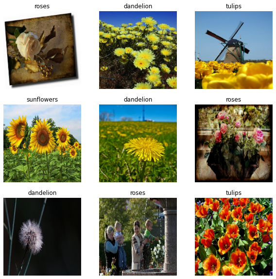
For classification models, we have a single label for each set of images in the same class. Annotations can be made very easily.
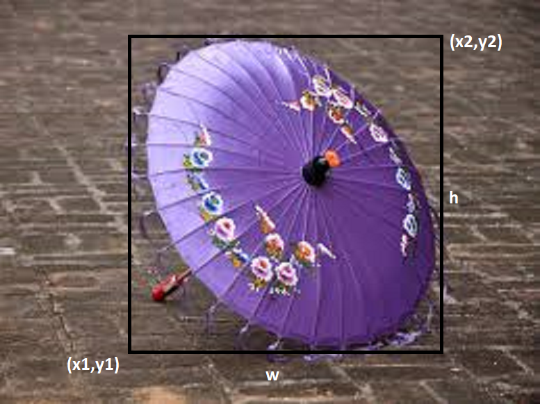
We usually use rectangular bounding boxes for object detection. Detection Models like YOLO and Faster-RCNN use this type of annotations. Bounding boxes are ususally represented by either the coordinates (x1,y1) lower left corner or (x2,y2) upper right corner of the box, followed by height and wigth of the bounding box.
Bounding boxes are simple but not ideal for all types of objects as we have to frame every object in a rectangular box. To solve this problem, polygonal segmentation is introduced. With this method, we can annotate the exact features of the objects with polygons. The image below is from one of my projects for segmentation of temples in ASEAN.

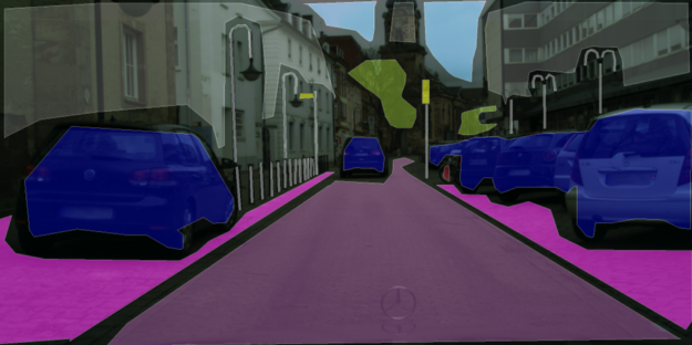
This technique takes segmentation to the pixel level. A particular class is assigned to every pixel in the image. Semantic segmentation is used mainly in situations where there is a very significant environmental context. It is used, for instance, in self-driving cars and robotics so that the models understand the environment in which they operate.
References
Tensorflow, Google images , Sabina Pokhrel's article , Cityscapes dataset