Week 2, Day 2 (Introduction to Artificial Intelligence and Computer Vision)
Welcome to second day (Week 2) of the McE-51069 course. In this week, we will walk you through with basic Knowledge on Deep learning and Computer Vision.
Review
In the last post, we introduce the basic components in building a neural network.
- Weights and Bias
- Activation Functions
- Loss Function
- Optimization (Gradient Descent)
And the process in which an input data pass through the network, calculating the loss is called the forward propagation and with that loss value update the model parameters is called backward propagation.
Adam Optimizer
Now, we will introduce Adam optimizer, which is also known as the adaptive moment estimation optimizer.
Let's recall the Gradient Descent Optimizer:
$W = W-\alpha \frac{dL}{dW}$, in which $\alpha$ is called the learning rate, which is a constance or decaying learning rate, depanding on the number of epoch trained.
The weight value is updated according to the loss value. But, the loss value from the model can be instable at first, due to dataset randomness, or dropout in model. So, instead of directly update the new $\frac{dL}{dW}$, we will update the exponentially weighted average of $\frac{dL}{dW}$, which state that, the model is updated according to the past and current $\frac{dL}{dW}$. The result is smoother update in the weight value respect to the loss.
$V_t = \beta*V_{t-1} + (1-\beta)dW$
$W = W - \alpha V_{dW}$
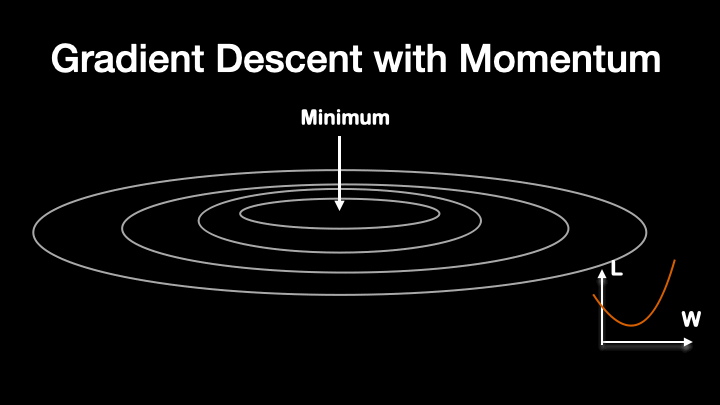
Like that, another method called RMS Prop further smooth out the training procedure.
$S_{dW} = \beta_2*S_{dW} + (1-\beta_2)dW^2$
$W = W - \alpha\frac{dW}{\sqrt{S_{dW}} + \epsilon}$
By combining the two equations above, the eqaution for Adam optimizer become:
$W = W - \alpha\frac{V_{dW}^{corrected}}{\sqrt{S_dW^{corrected} }+ \varepsilon}
$
There are two hyper-parameters in this equation and the author of the adam optimizer suggests the value for $\beta_1$ to be 0.9 and $\beta_2$ to be 0.99.
Dataset
There are two main factors in making a great AI model.
- The algorithms (model architecture, loss function, optimizer)
- Dataset or environment in reinforcement learning.
Dataset is like the fuel for our model. If the dataset is well processed, and contain rich information, the performance of the model can go up accordingly.
When we get a dataset and want to use it for training the model, we will first have to separate the dataset into three parts:
- Training Dataset (Dataset used to train the model)
- Validation Dataset (Dataset used for hyper-parameters tunning)
- Testing Dataset (Dataset used for evaluating model performance)
Train / Validation / Test
Today is a big data era, where we can easily get accessed to millions of dataset. Typcially, when training a small simple network, a small dataset is enough, but with deep learning, we can construct more complex model with ease and so the need for data is becoming larger and larger. Typically, we can divide these data into 3 parts with each percentage of 70/15/15. But, if the dataset is large, let's say 60,000 images in CIFAR10 dataset, 10 percent of the dataset already contain 6,000 images. And that is enough to test our model performance. So, we often divide the dataset into 80/10/10. But it is up to you.
Bias and Variance
Clean and well structured data can help model to learn faster and better. But in real world, it is really hard to get dataset that is clean. Often, what we have to encounter are the datasets that have outliers, wrong data point. So, when training, we want our model to be robust of such outlier. For that, we will introduce two ideas: Bias and Variance.
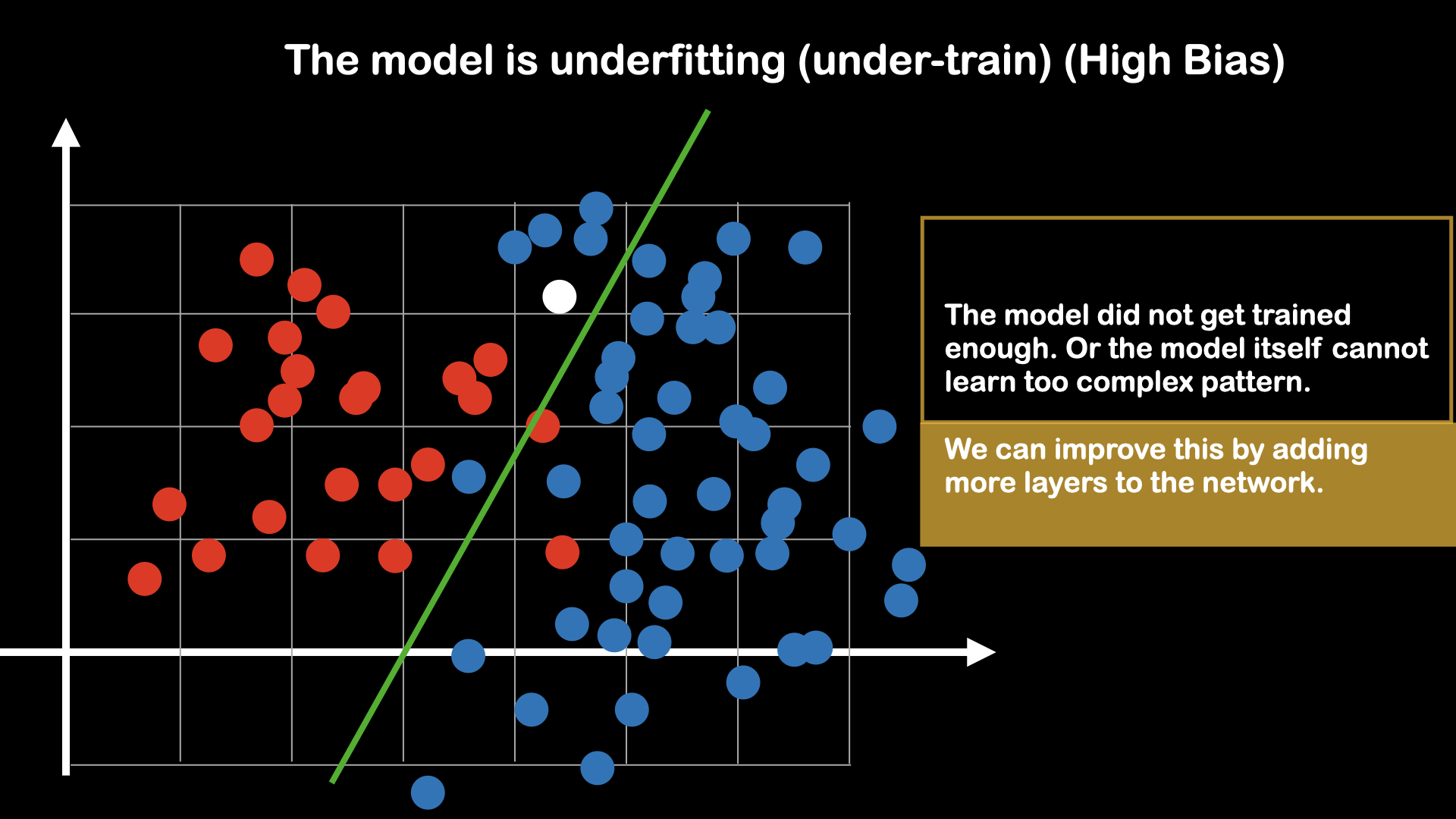 Fig : Model is undertrain
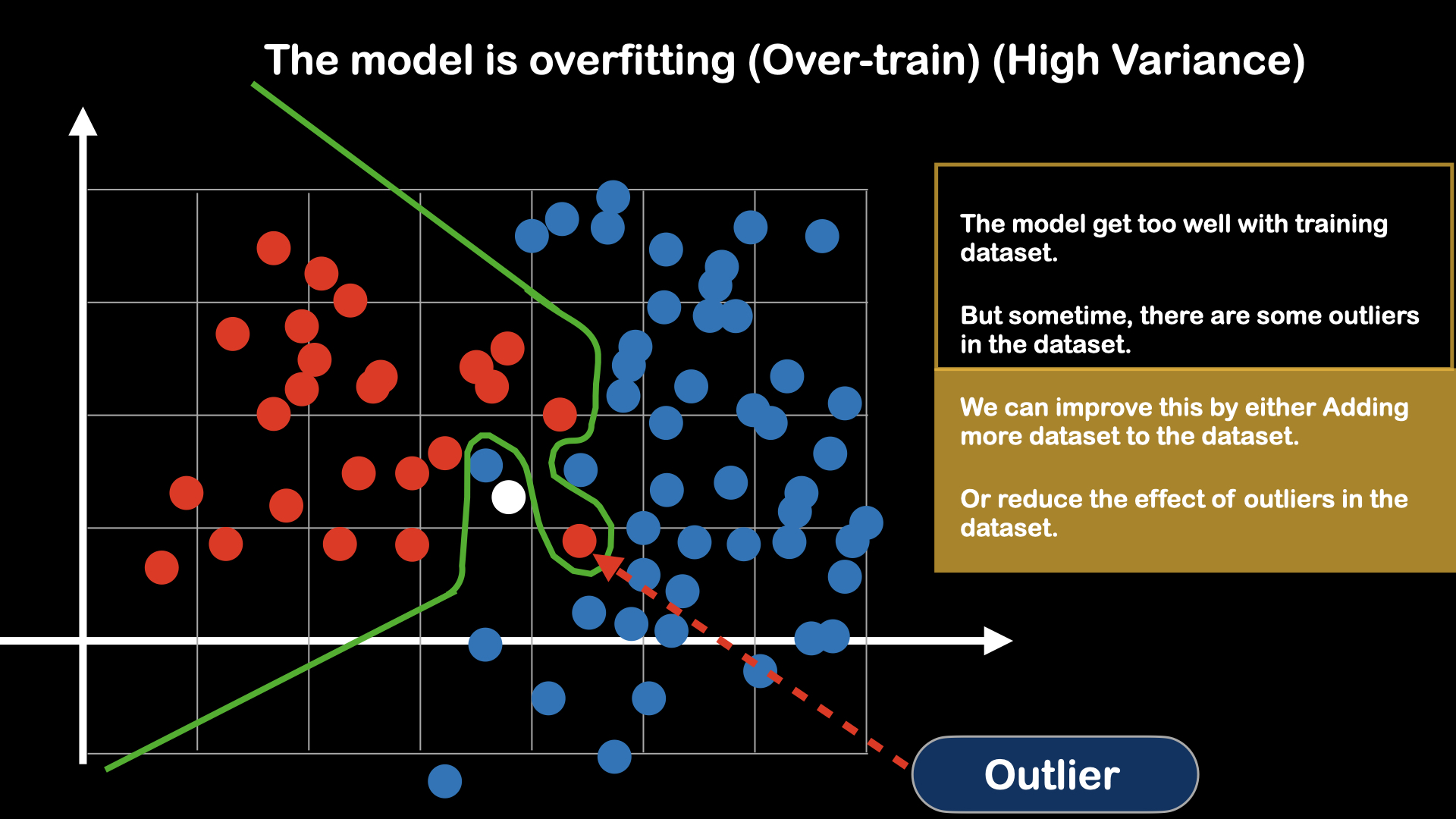 Fig : Model is overtrain
Regularization
Underfitting can be solved by simply making the model to be more complex (adding more layers), able to learn non-linearity. But, regarding about the overfitting, we have to make adjustment, either to the model, or to dataset. This process of preventing the overfitting of the model is called regularization.
Typical regularization methods contain:
- Model side:
- L1 and L2 regularization
- Drop out
- Dataset side:
- Data Augmentation
The regularization on the model side, is basically making the model to be simple, opposite to fixing underfitting problem, by turning some neurons in the model off. We will discuss more about regularization method in the following section.
$L_1$ and $L_2$ Regularizaiton
$L_1$ and $L_2$ regularization is done by adding penalty to the cost function: $J$
The original cost function is:
$J = \frac{1}{m}\sum_{m=0}^i L$
In $L_1$ regularization, the cost function is modified to :
$J = \frac{1}{m}\sum_{m=0}^i (L +\frac{\lambda}{2m}W) $
In $L_2$ regularization, the cost function is modified to :
$J = \frac{1}{m}\sum_{m=0}^i (L +\frac{\lambda}{2m}W^TW) $
To reduce the cost value, the regularization part must be kept small, and so the weight value will be small or kept to zero, which is the same as turning the neuron cell off.
Dropout and Cutout
Dropout is one of the most commonly used method for regularization. Here, we will take cutout as example and explain why dropout work.
Neural network work by detecting the features in the dataset. And since some of the features are more importance than the others, the neural network tends to focus more on these features and ignore other features. That may lead to bias, biased to some features in the dataset.
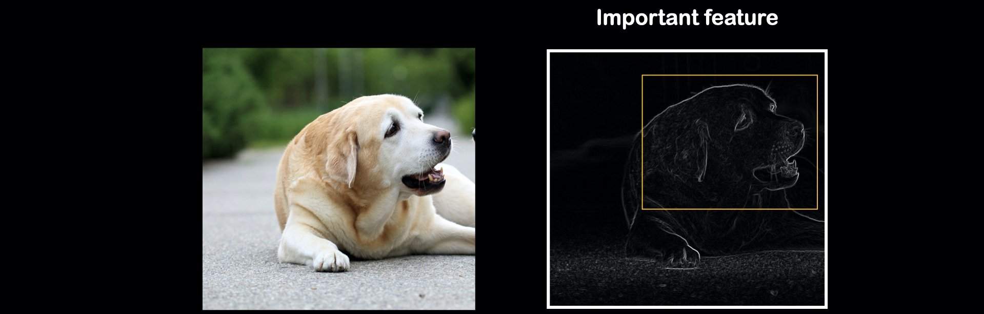
Like the figure show above, the model will most likely focus on the face part of the dataset. To avoid that, when training, we can introduce some random cutout of the dataset. Cutout is the data augmentation method, in which random part of the input are being cropped out.
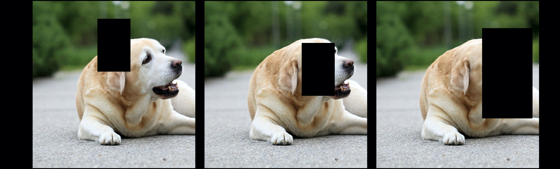
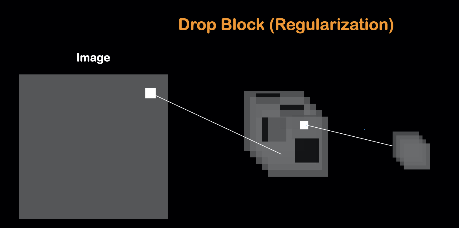
This way, our model is forced to learn other features aside from the most importance feature. This is on the dataset side. For the model side, this is carried out by dropout, which randomly shut down some of the neurons in training process. In convolutional neural network, this process is called dropblock.
Data Augmentation
Data augmentation is one of the most used regularization method. And this method can greatly effect model training performance. Data augmentation means making extra dataset from the existing dataset. For example, in image dataset, even thought the object in the image is the same, the pixel position, the pixel value can change dramatically. By the methods to augment the data, it can be divided into two types:
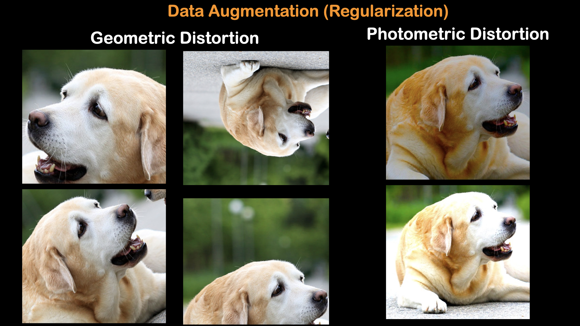
Geometric distortion is achieved by changing the pixel coordinates: Rotation, Translation. Photometric distortion is achieved by changing the pixel value: Contrast, Brightness, etc.
Framework
There are many frameworks for building the deep learning model. In this course, we will use Pytorch, which is a open source machine learning library based on Torch library. Pytorch has recently gain more popularity with researchers and in production lines. So, there are many resources for learning deep learning model. And it is more friendly than tensorflow, which is also a open source deep learning library.
Platform
For training a deep neural network, it is better to have a GPU for faster training.
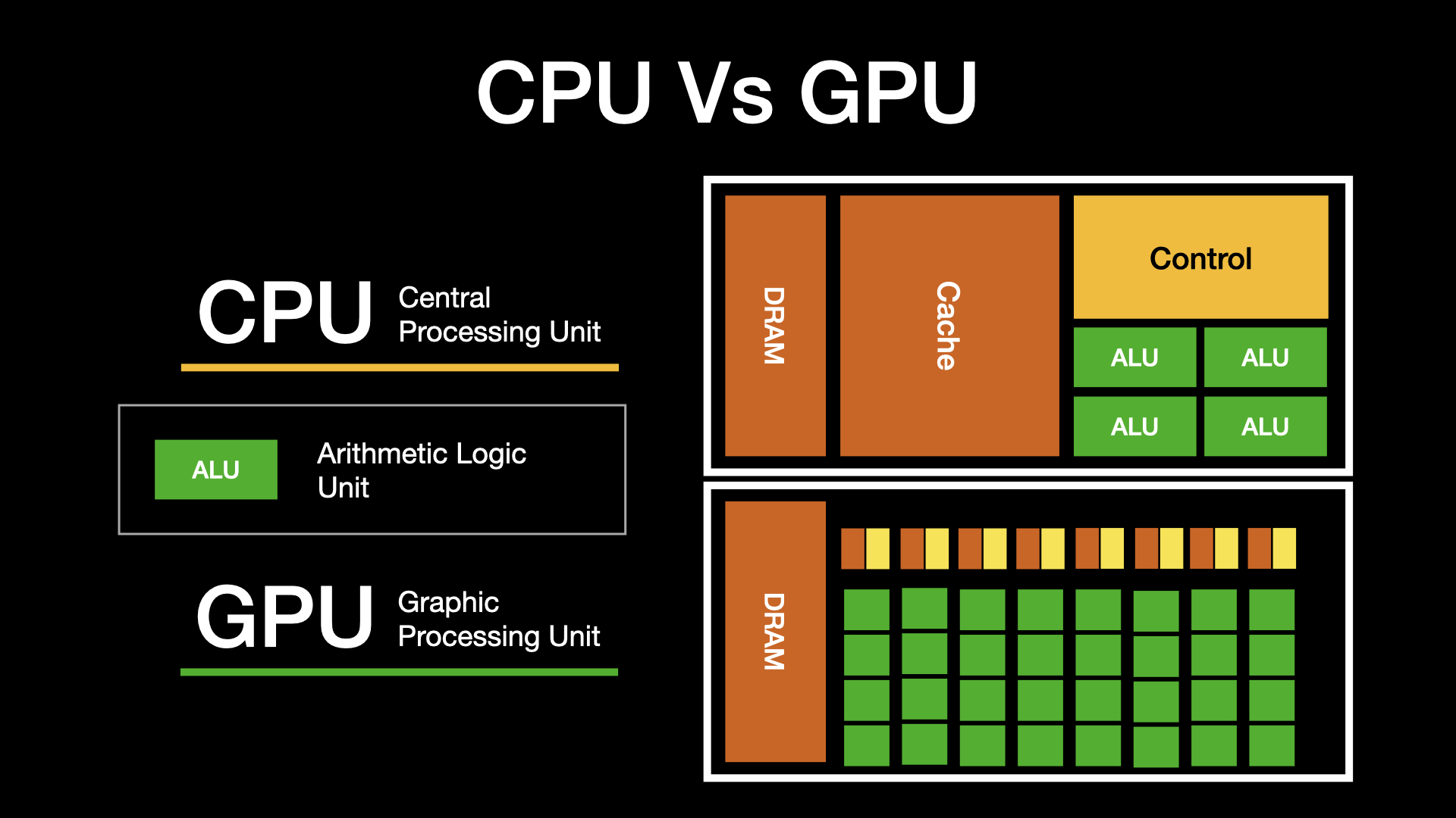
GPU, which can process more parallel task than CPU, are great arsenel in training neural network. And because not all students have a descent GPU in their comptuer, we will use google colaboratory, which is a jupyter-like development platform where we can get accessed to free GPU.