Week 2, Day 1 (Introduction to Artificial Intelligence and Computer Vision)
Welcome to first day (Week 2) of the McE-51069 course. In this week, we will walk you through with basic Knowledge on Deep learning and Computer Vision.
- Artificial Intelligence
- Computer Vision
- AI Today
- Neural Network
- Deep Neural Network
- Conclusion
- Further Resources
Artificial Intelligence
Human has always been fascinated by the ideas of putting the intelligence to the machine. Still, it was until 1956, the term "Artificial Intelligence" was coined, at a conference at Dartmouth College, in Hanover, New Hampshire. At such time, people were very optimistic about the future of AI. And the fundings and interest invest in the field get larger and larger.
But making a machine to behave just like a human is not an easy task. With the researchers fail to deliver the promise, and also with several reports criticizing progress in AI, the funding and interest in the field get dropped off, people later often refers this as the "AI winter" which happend during 1974s-1980.
Even though there are some private and public fundings to the field, the whole hype about "Aritificial Intelligence" gets cooled down. At around 1987s to 1993, the field experienced another "winter".
It was only after 1997, IBM's Deep Blue became the first computer to beat a chess champion, Russian grandmaster Garry Kasparov, that the term "AI" was again coming back to the reserach ground.
The field of artificial intelligence finally had its breakthrough moment in 2012 at the ImageNet Large Scale Visual Recognition Challenge (ILSVRC) with the introduction of Alex-Net. (ILSVRV) is a vision competition and before Alex-Net, the error rate in this competition hover around 26%. But with Alex-Net, the error rate comes down to only 16.4%. That is a huge accomplishment and people now see hope in Deep Neural Networks Again.
Nowaday, when people talk about "Artificial Intelligence", they often refers to "Deep Neural Networks", a branch of Machine learning that imitates the human brain cells as to function and process data. And with modern hardware advanced, big data accessable and algorithms optimized, the field of Deep Learning is getting more and more research interestes and improvements everyday.
Computer Vision
The main purpose of computer vision is for computer to have the "vision", ability to perceive the world, like we human do. To do that, we have to know how human vision system work. It is now known that, human vision is hierarchical, a step by step procedure. Neurons detect simple features like edges, and then recognite more complex features like shapes, and then eventually see the whole complex visual representations.
 source :
 Today, we have the AI algorithms, that mimic the hierarchical architecture of the human vision system called the CNN(Convolutional Neural Networks). CNNs use convolutional layers to extract the features in images and then use fully connected layers for the output.
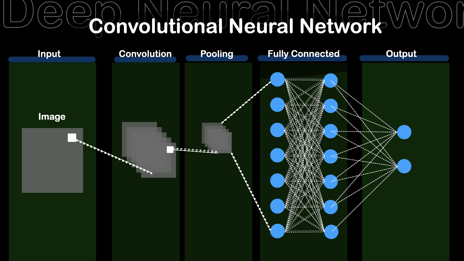 Fig : Simple Convolutional Neural Network
AI Today
Even though many people think that AI is still far away from our daily life, it is not quite true. When we surf on social media, let's say Facebook, we get the newsfeed from Facebook's recommandation AI. And when we travel using "Google Maps", it automatically generates the traffic conditions using AI. What we didn't realize is, AI has already been a part of our daily life and improving our living quality.
Neural Network
Neural Network is the basic building block for the Deep Neural Networks. It behave like the neuron cell in our brain. It receive information, process it and feed into next cell, and form the network.
We will walk you through step by step how a neural network is constructed.
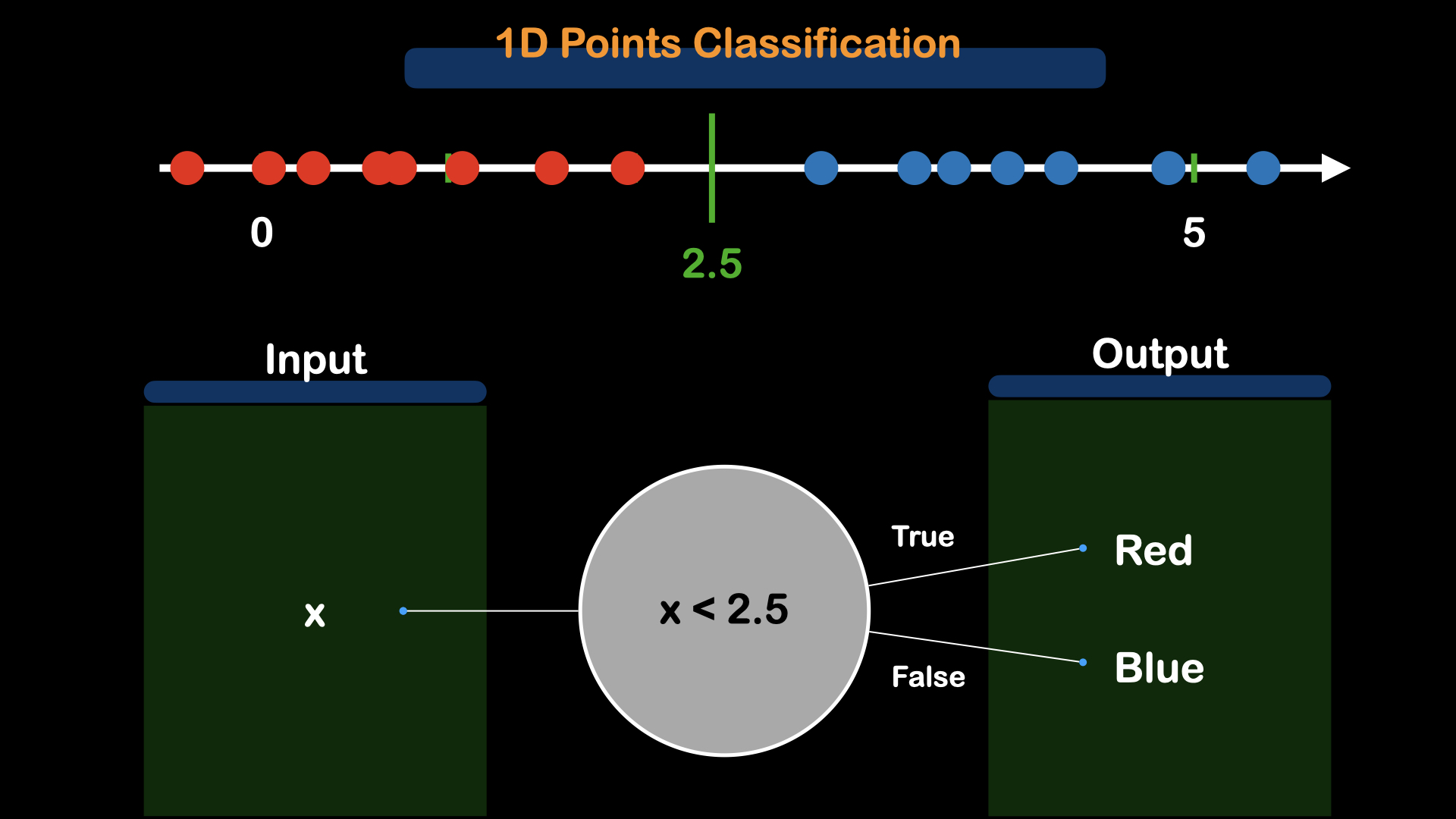
Let's first do a simple classification on two data points.
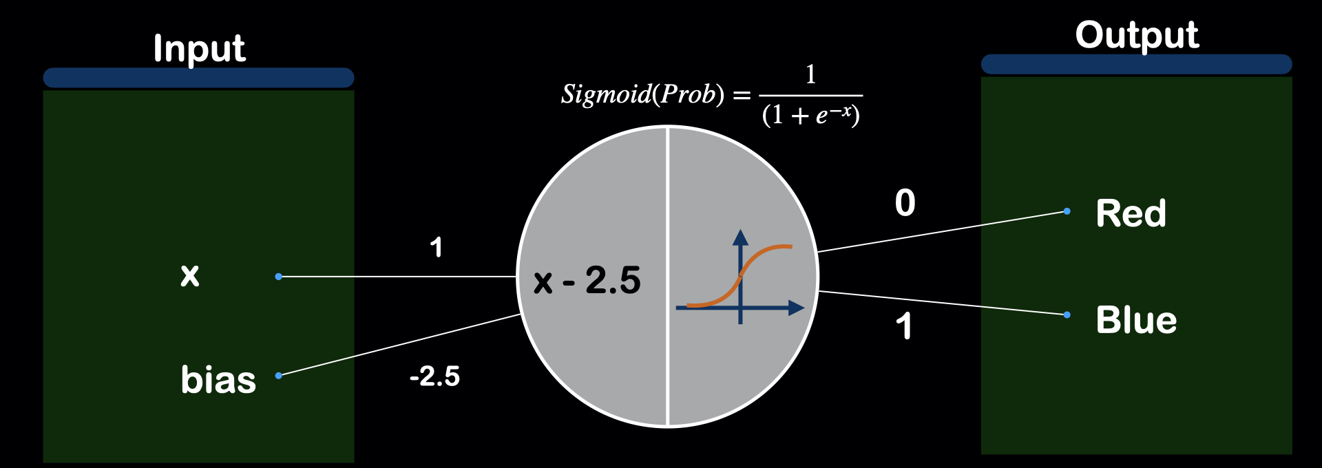
Given the x-coordinate of the data point, we will have to classify wherether this point belongs to red or blue. For that, we will need to find the threshold value, decision boundary or decision surface, whatever you may call it. For this particular example, the threshold value would be 2.5.
So, we can write this with the logic of taking x-coordinate as the input,x, and check if it is smaller than 2.5, if True, then, the color is "Red", and if False, the color is "Blue".
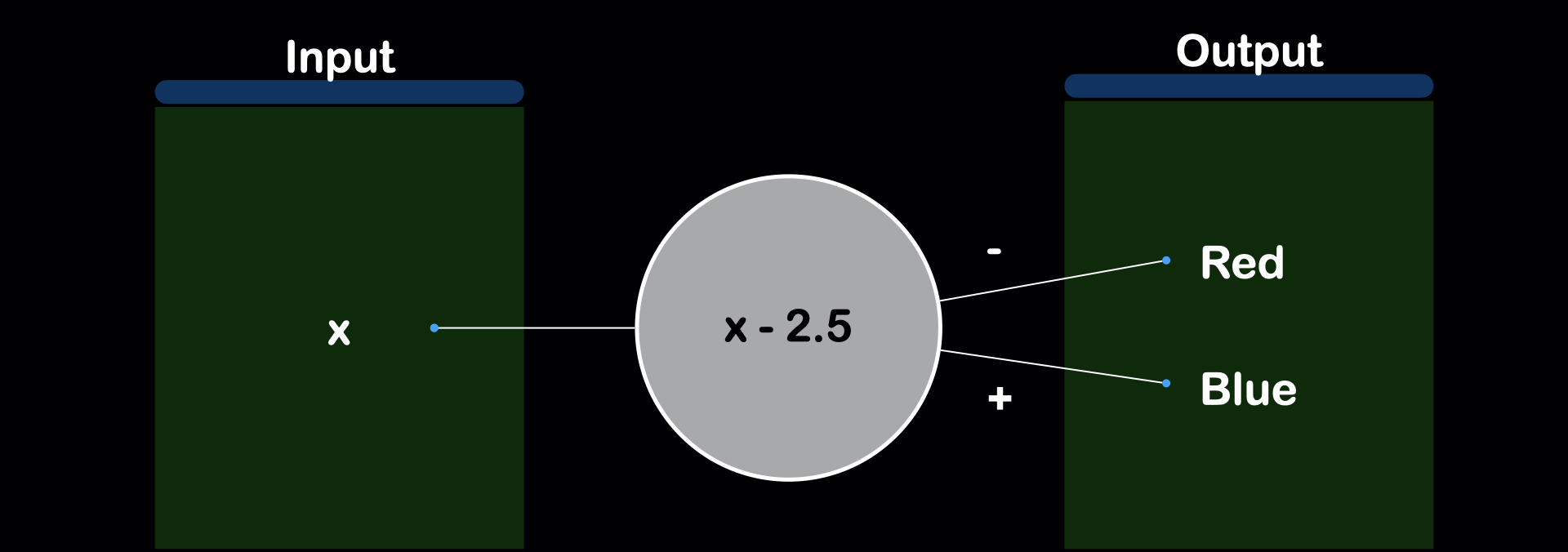
We can also write the function instead of logic with x-2.5, and check if positive or negative.
But, still, we do not know the confidence of prediction value by the above equation. For example, for a point that have x_coordinate of 3, it should have a probability of being blue for around 60%, and for point that have x_coordinate of 100, it should be 100% blue point. To convert to the probability value, Sigmoid function is introduced. It keeps the output range from 0~1. So, if the output from sigmoid is near 1, let's say, 0.9, we would say that this point is 90% sure to be the "Blue" Point. And if the output from the sigmoid is 0.2, we would say this point is 20% sure to be the "Blue" Point or (1-0.2 = 0.8) 80% sure to be the "Red" Point.
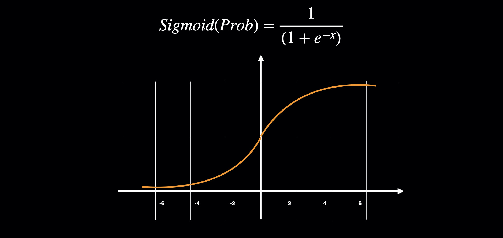 Fig : Sigmoid function keep output value from 0 to 1
We add sigmoid function at the output of the function, outputing the probability of the point being blue.
Next, let's apply this logic with 2 dimensions(x and y).
Remember when we introduced the threshold value, we refered the point as the decision boundary or decision surface. That is because that value(threshold) makes the decision for the model in a single dimension.
For 2 dimensional cases, we will need a Line (2D) instead of Point (1D) as a decision boundary for classification.
So, as the dimension for the dataset increases, the dimension of the decision surface also increases.
In 1D : $(x-2.5)$ : Only 1 variable (Point)
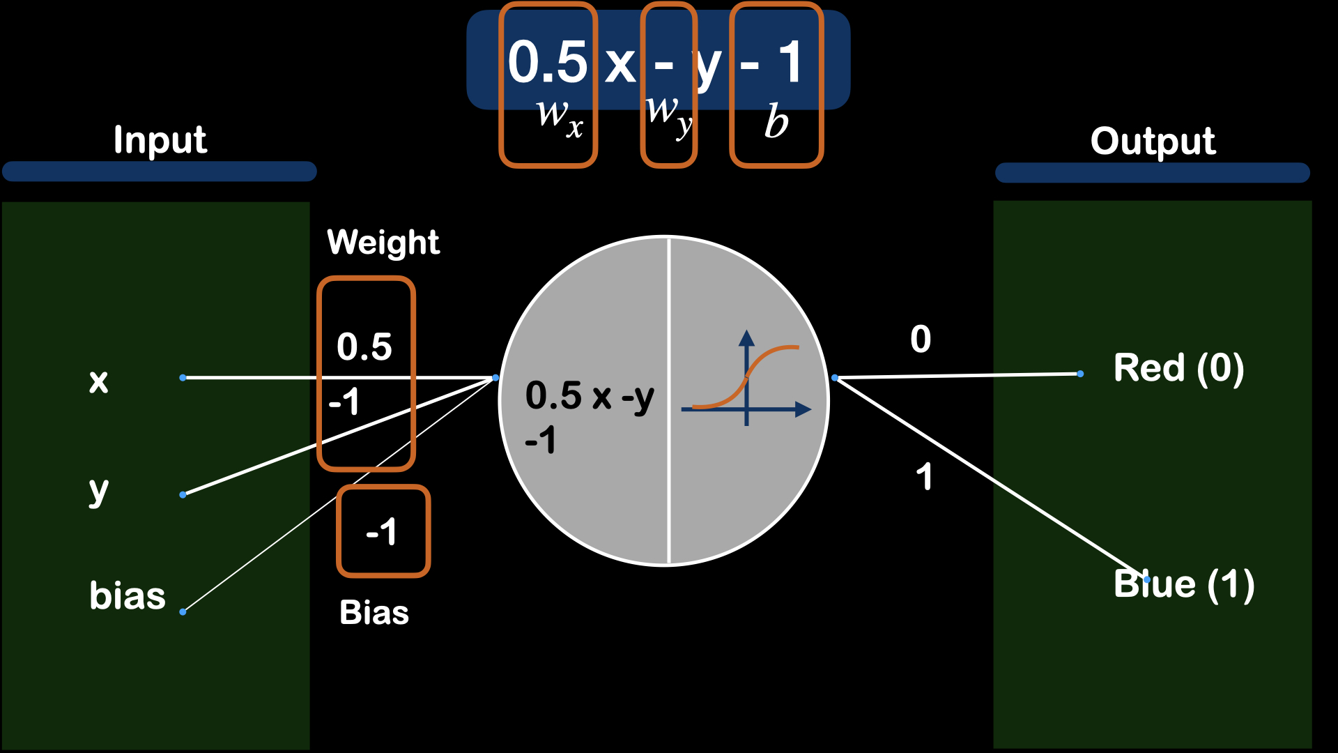
In 2D : $(0.5x -y -1)$ : 2 variables (Line)
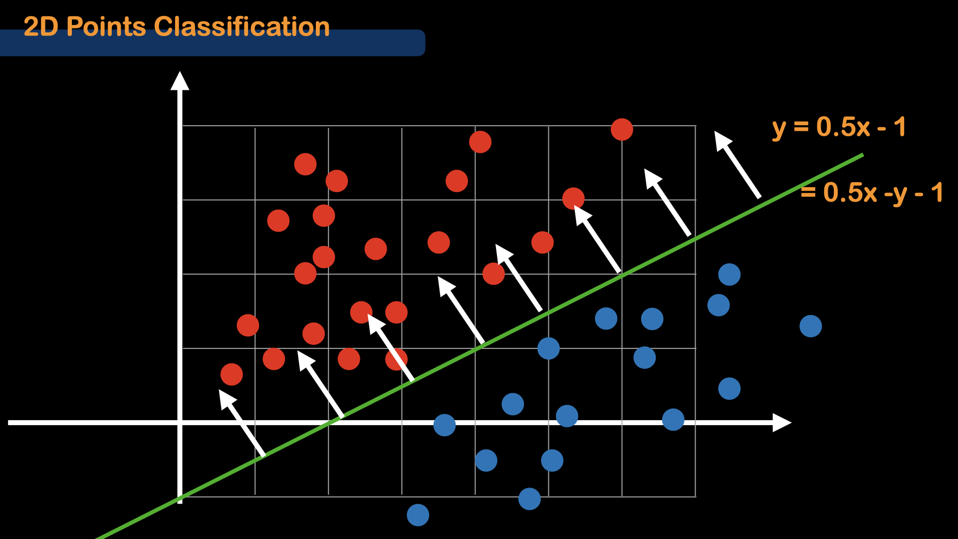
For this particular example, let's say, the equation for the line is $ y = 0.5x - 1$, then, it can be derived to $ 0.5x - y - 1$. Here, we introduce "Weight", the coefficient of variables, and "Bias", which is a constant value.
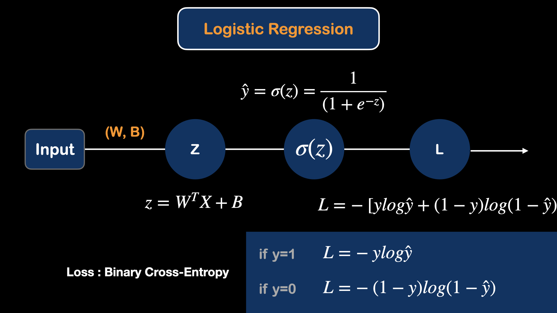
And with the extra loss function, the basic logistic regression model is developed. Loss function for the model determines how badly the model is performing. And the model is updated according to the loss value, large loss value will lead to large update in model parameters(weights) and small loss value indicate better performace of model and will lead to small update in model parameters(weights). There are many loss functions for different task and different loss function can effect the model performace in training. For this particular case, we will use "Binary cross-entropy" Loss.
After finding the Loss of the model, We would like to update(optimize) the model. Updating model parameters for better performace is called optimization. To optimize the model, gradient descent method will be introduced.
First, the variables(parameters) that we can update in the model are "weight" and "bias". So, we need to know, how the change in weight effect loss. Mathematically, this is called the derivative.
So, we would like to know $ \frac{dL}{dW}$.
And since the equation for the loss is:
$L = -[ylog\hat{y} + (1-y)log(1-\hat{y})]$
| Equation | Depandance |
|---|---|
| Loss Equation above | L depends on $\hat{y}$ |
| $\hat{y} = \sigma{z}$ | $\hat{y}$ depends on z |
| $Z = W^TX + B$ | Z depands on W |
We can use chain Rule to find the derivative of L respect to W with the following equation.
$\frac{dL}{dW} = (y - \hat{y}) * X$
If you would like to see the derivation steps, here is this link from stack exchange.
After that, we can update the weight values with gradient descent equation:
$W = W - \alpha \frac{dL}{dW}$
$\alpha$ here means the learning rate, which is a hyperparameter we can adjust to get the better convergence rate for the model.
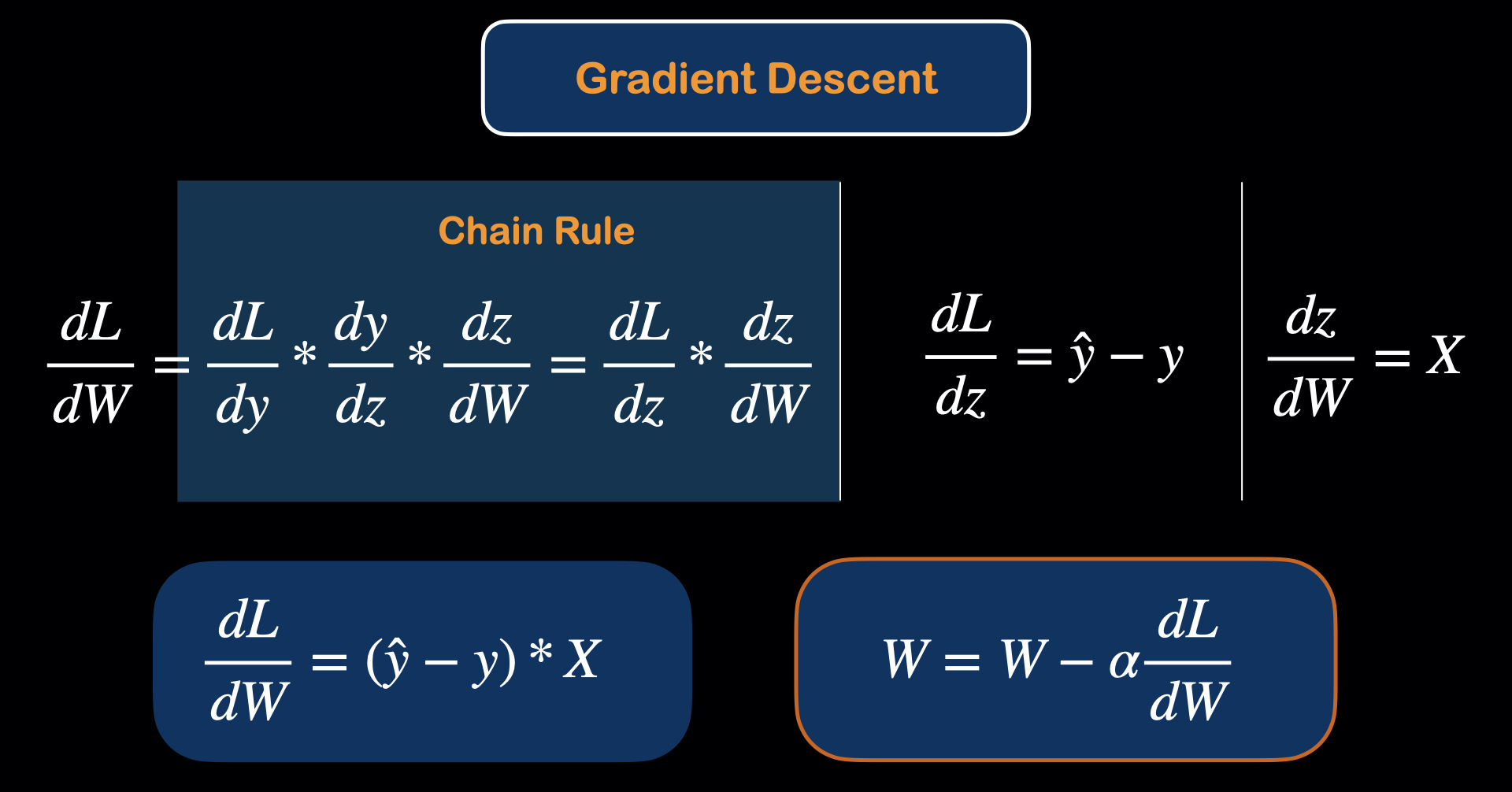
The way that Gradient Descent work is that it changes the model parameter in such a way to get minimal loss value.
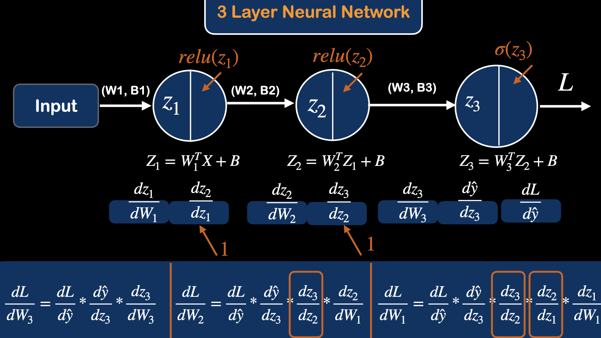
Deep Neural Network
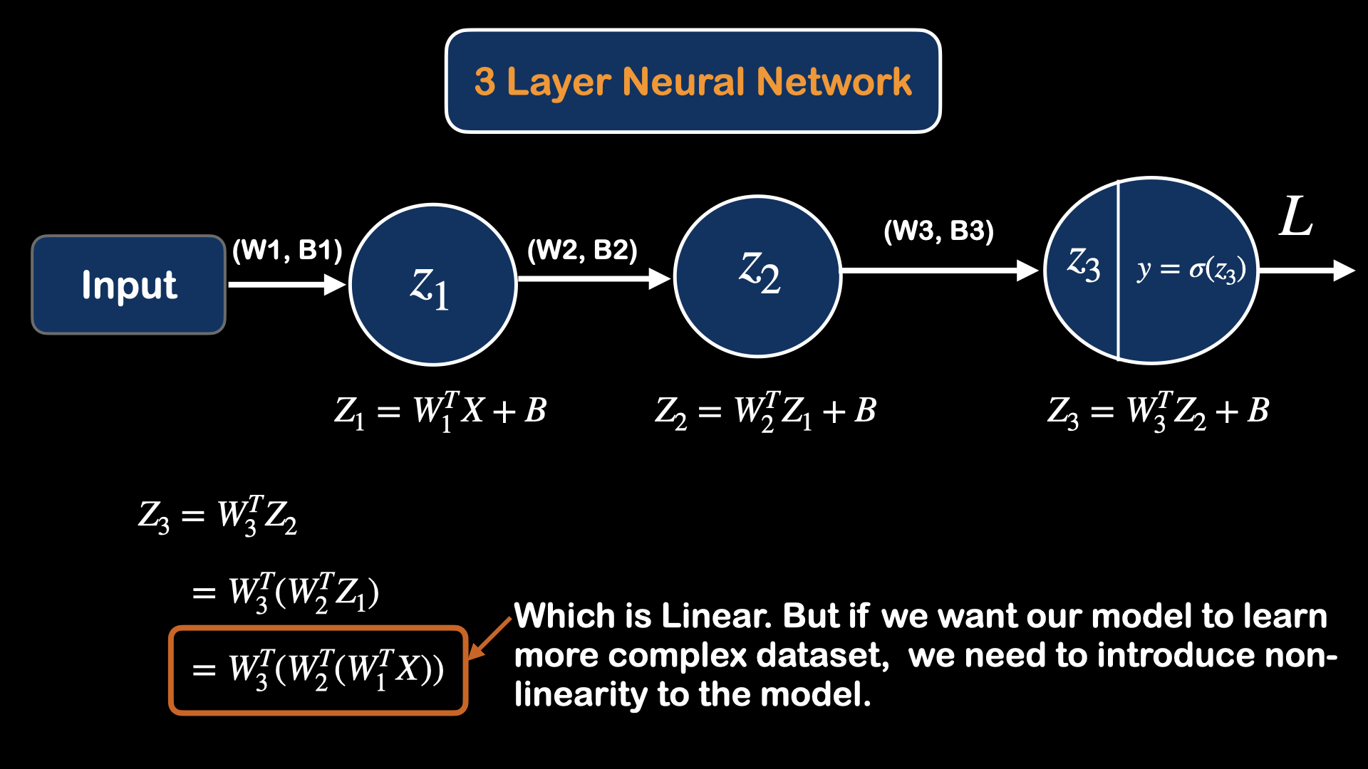
What happens if we add more units of cells to the previous model?
The main problem with just simply stacking cells is that the model is still acting linearly. So, we need to introduce some kind of non-linearity to the model, by adding "activation function" to each output of the cell.
Now, we will introduce Relu (Rectified Linear Unit), which behaves just like linear function if the output is higher than 0.
The equation for the relu function is as follow:
$relu(z) =
\begin{cases}
z & if\ z>0\\
0 & if\ z<=0
\end{cases}$
And the derivative for the relu is
$\frac{d}{dz}relu(z) =
\begin{cases}
1 & if\ z>0\\
0 & if\ z<=0
\end{cases}$
The main advantage of using relu is that it does not activate all the neurons at the same time. When the value of z is negative, relu turns it off, returning the zero value, indicating that this feature is not important for the neurons to learn. And since only a certain number of neurons get activated, it is far more computationally efficient than sigmoid and other activation functions.
If you would like to learn more about various Activation functions, please visit this blog post for more details.
Further Resources
If you would like to learn more about neural networks, you can visit Deeplearning.ai on youtube.